")
")
")
")
Kinetic theory of gases
- Details
- Written by: Germán Fernández
- Category: Kinetic theory of gases
- Hits: 1528
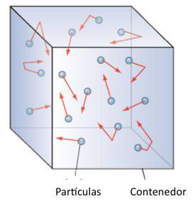
The kinetic theory of gases allows deducing the properties of the ideal gas using a model in which the gas molecules are spheres that comply with the laws of classical mechanics.
The properties that can be calculated using this model are: gas pressure, molecular velocity distribution, mean molecular velocity, collision velocity, and mean distance between collisions. These properties allow the study of the kinetics of reactions in the gas phase as well as the flow of fluids and heat transfer.
Fundamentals of the kinetic-molecular theory of gases
 Kinetic theory can be considered as a branch of statistical thermodynamics since it deduces macroscopic properties of matter from molecular properties. The principles on which it is based are the following:
- A gas is made up of a large number of spherical particles whose size is negligible compared to the distance between the particles.
- Molecules move in straight lines at high speed and only interact when they collide. The collisions between particles and with the walls of the container are considered perfectly elastic, conserving the translational kinetic energy.
- Kinetic theory assumes that particles obey Newton's laws. This assumption is incorrect (molecules obey the laws of quantum mechanics) and leads to incorrect results in predicting the heat capacities of the gas, although it gives acceptable results in properties such as pressure or diffusion.
- Details
- Written by: Germán Fernández
- Category: Kinetic theory of gases
- Hits: 1494
The speed distribution functions will allow us to know the fraction of molecules with speeds between two given values.
We are going to use 3 distribution functions:
- For the velocity components $g(v_x),g(v_y)$ and $g(v_z)$.
- For the velocity vector $\phi(\vec{v})$
- For the velocity module $G(v)$.
Distribution functions of the velocity components $g(v_x),g(v_y)$ and $g(v_z)$
The distribution function $g(v_x)$ allows to know the fraction of molecules with velocities between $v_x$ and $v_x+dv_x$.
\begin{equation} dN_{v_{x}}/N=g(v_x)dv_x \end{equation}
Analogous equations can be written for the distribution functions in the y,z direction
\begin{equation} dN_{v_{y}}/N=g(v_y)dv_y \end{equation}
\begin{equation} dN_{v_{z}}/N=g(v_z)dv_z \end{equation}
- Details
- Written by: Germán Fernández
- Category: Kinetic theory of gases
- Hits: 1562
The probability of finding a molecule at a given energy level, j, is given by:
\begin{equation} p_j=\frac{e^{-\epsilon_j/kT}}{\sum e^{-\epsilon_i/kT}} \end{equation}
From the classical point of view, the kinetic energy of a molecule varies continuously and is given by the expression $\epsilon_x=\frac{1}{2}mv_x^2$. Taking this energy value to the probability expression, we obtain:
\begin{equation} dp(v_x)=\frac{dN_{v_x}}{N}=\frac{e^{-\frac{mv_x^2}{2kT}}dv_x}{\int_{-\infty} ^{\infty}e^{-\frac{mv_x^2}{2kT}}dv_x} \end{equation}
Where, $dp(v_x)$ represents the fraction of molecules with speed between $v_x$ and $v_x+dv_x$. The integral of the denominator represents the sum over all possible values of $v_x$ and has the form $\int e^{-bx}dx=(\pi/b)^{1/2}$
\begin{equation} dp(v_x)=\frac{dN_{v_x}}{N}=\frac{e^{-\frac{mv_x^2}{2kT}}dv_x}{\left(\frac{2 \pi kT}{m}\right)^{1/2}} \end{equation}
Given that $\frac{dN_{v_x}}{N}=g(v_x)dv_x$, the distribution function for $v_x$ is given by:
\begin{equation} g(v_x)=\left(\frac{m}{2\pi kT}\right)^{1/2}e^{-mv_{x}^{2}}/2kT \end{equation}
where m is the mass of a gas molecule, k is Boltzmann's constant, and T is the temperature.
Read more: Obtaining the distribution function for $v_x$ $g(v_x)$
- Details
- Written by: Germán Fernández
- Category: Kinetic theory of gases
- Hits: 1409
The probability that a molecule has its velocity component in the x-direction between $v_x$ and $v_{x+dx}$, in the y-direction between $v_y$ and $v_{y+dy}$, and in the z-direction between $v_z$ and $v_{z+dz}$ will be given by: \begin{equation} dN_{v_x,v_y,v_z}/N=g(v_x)g(v_y)g(v_z)dv_xdv_ydv_z \end{equation} $dN_{v_x,v_y,v_z}/N$ represents the probability that a molecule (fraction of molecules) has the end of its velocity vector inside a box with sides $dv_x, dv_y, dv_z$
Substituting the expressions computed above for the distribution functions in each spatial direction: \begin{equation} \phi(\bar{v})=g(v_x)g(v_y)g(v_z)=\left(\frac{m }{2\pi kT}\right)^{1/2}e^{-mv^2/2kT} \end{equation} Where, $v^2=v_x^2+v_y^2+v_z^2$ , the square of the magnitude of the velocity. This new distribution function does not depend on the orientation of the vector, but exclusively on its magnitude.
- Details
- Written by: Germán Fernández
- Category: Kinetic theory of gases
- Hits: 1520
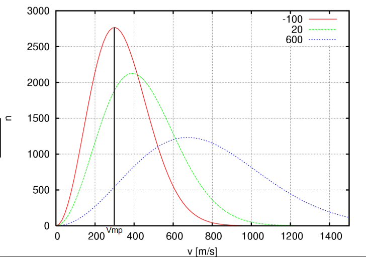
In this section we are going to deduce the equation that allows us to know the fraction of molecules that have the magnitude of their velocity between two determined values.
We call $dN_v/N$ the fraction of molecules with speed between v and v+dv. where N represents the total number of gas molecules. \begin{equation} \frac{N_v}{N}=G(v)dv \end{equation} G(v) is the velocity distribution function or probability density. By multiplying this function by $dv$, the fraction of molecules with speed between v and v+dv is obtained.
If we are interested in calculating the fraction of molecules with a velocity between $v_1$ and $v_2$, we integrate the velocity distribution function in that interval. (It is equivalent to talk about the fraction of molecules that have their speed in a given interval and the probability that a molecule has its speed included in said interval)
\begin{equation} P[v_1,v_2]=\int_{v_1}^{v_2 }G(v)dv \end{equation}
The probability that a molecule has its speed in the interval $[0,\infty]$ is 1
\begin{equation} \int_{0}^{\infty}G (v)dv=1 \end{equation}
Read more: Obtaining the distribution function of the velocity module $G(v)$
- Details
- Written by: Germán Fernández
- Category: Kinetic theory of gases
- Hits: 1622
\begin{equation} \bar{v}=\int_{0}^{\infty}vG(v)dv=4\pi\left(\frac{m}{2\pi kT}\right)^{3 /2}\int_{0}^{\infty}e^{-mv^2/2kT}v^3dv \end{equation} Using the integral $\int_{0}^{\infty}x^{2n+ 1}e^{-ax^2}dx=\frac{n!}{2a^{n+1}}$ \begin{equation} \bar{v}=4\pi\left(\frac{m} {2\pi kT}\right)^{3/2}\frac{1}{2(m/2kT)^2}=\left(\frac{8kT}{\pi m}\right)^{1 /2} \end{equation} Multiplying and dividing by Avogadro's number and taking into account that $kN_A=R$ and $N_A m=M$ \begin{equation} \bar{v}=\left(\frac{ 8RT}{\pi M}\right)^{1/2} \end{equation}
- Details
- Written by: Germán Fernández
- Category: Kinetic theory of gases
- Hits: 1472
The most probable speed is the speed at which the function G(v) is maximum and is obtained by setting the derivative of G(v) with respect to v to zero. \begin{equation} \frac{dG(v)}{dv}=0\;\;\rightarrow \;\;v_{mp}=\left(\frac{2RT}{M}\right)^{1 /2} \end{equation}
- Details
- Written by: Germán Fernández
- Category: Kinetic theory of gases
- Hits: 1409
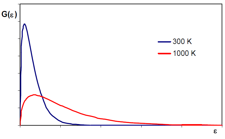
The Maxwell distribution can be written in terms of translational energies $\epsilon_{tr}=\frac{1}{2}mv^2$, solving for v, $v=\left(\frac{2\epsilon_{tr}} {m}\right)^{1/2}$, differentiating: \begin{equation} dv=\left(\frac{2}{m}\right)^{1/2}\frac{1}{2 }\epsilon_{tr}^{-1/2}d\epsilon_{tr}=\left(\frac{1}{2m}\right)^{1/2}\frac{d\epsilon_{tr}} {\epsilon_{tr}^{1/2}} \end{equation} Substituting vy dv into $\frac{dN_v}{N}=\left(\frac{m}{2\pi mkT}\right)^ {3/2}e{\frac{-mv^2}{2kT}}4\pi v^2dv$ \begin{equation} \frac{dN_{\epsilon_{tr}}}{N}=\left( \frac{m}{2\pi mkT}\right)^{3/2}e^{\frac{-m(2\epsilon_{tr}/m)}{2kT}}4\pi \left(\ frac{2\epsilon_{tr}}{m}\right)\left(\frac{1}{2m}\right)^{1/2}\frac{d\epsilon_{tr}}{\epsilon_{tr }^{1/2}} \end{equation} Simplifying: \begin{equation} \frac{dN_{\epsilon_{tr}}}{N}=2\pi \left(\frac{1}{\pi kT}\right)^{3/2}e^{\frac{-\epsilon_{tr}}{kT}\epsilon_{tr}^{1/2}}d\epsilon_{tr} \end{equation} $dN_{\epsilon_{tr}}$ represents the number of molecules whose translational energy is comp rendered between $\epsilon_{tr}$ and $\epsilon_{tr}+d\epsilon_{tr}$
The mean translational energy is the same for all gases at the same temperature.
- Details
- Written by: Germán Fernández
- Category: Kinetic theory of gases
- Hits: 2583
We are going to calculate the collision frequency of gas molecules with the wall of a container in a dt.
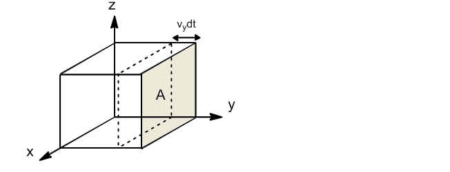
If we take the wall perpendicular to the y-axis, only molecules with velocity component y will collide against the wall. The fraction of molecules with component y of velocity between $v_y$ and $v_y+dv_y$ is given by:
\begin{equation} \frac{dN_{v_y}}{N}=g(v_y)dv_y \end{equation}
Only the molecules that are at a distance $v_ydt$ from the wall will be able to collide against it in the dt. The volume of the box in which the molecules that can hit the wall are found will be: $V'=Av_ydt$. Dividing this volume by the total $V'/V$, the fraction of molecules that due to their proximity to the wall can collide is obtained.
- Details
- Written by: Germán Fernández
- Category: Kinetic theory of gases
- Hits: 1735
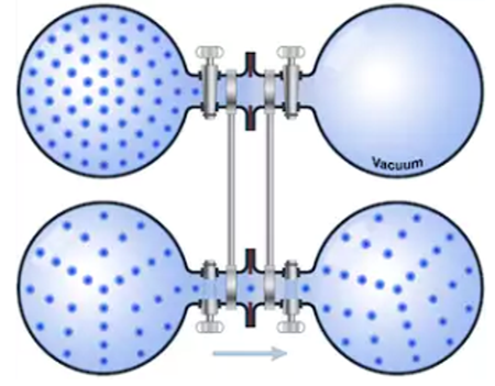
If a container containing a gas has a small hole of area $A_{or}$ and there is a vacuum outside the container, the molecules that collide with the hole escape from the container at a speed given by:
\begin{equation} \frac{dN}{dt}=\frac{-A_{or}P}{\left(2\pi mkT\right)^{1/2}} \end{equation}
The minus sign indicates that the molecules come out of the container. This phenomenon is called effusion, the effusion rates being inversely proportional to the square roots of the molecular masses.
- Details
- Written by: Germán Fernández
- Category: Kinetic theory of gases
- Hits: 1489
The vapor pressure of a liquid is measured by determining the rate of effusion of the gas in equilibrium with it. To do this, the weight loss w in the interior due to the escaping molecules is measured.
\begin{equation} \frac{dw}{dt}=m\frac{dN}{dt}=-\frac{A_{or}P_vm}{(2\pi mkT)}^{1/2}=- P_vA_{or}\left(\frac{m}{2\pi kT}\right)^{1/2} \end{equation}
In a finite time interval $\Delta t$, the following loss of weight:
\begin{equation} \Delta w=-P_vA_{or}\left(\frac{m}{2\pi kT}\right)^{1/2}\Delta t \end{equation}
Weighing the container at the beginning and at the end of the experiment we determine $\Delta w$ and using the previous equation the vapor pressure.
\begin{equation} P_v=\frac{\Delta w}{A_{or}\Delta t}\left(\frac{2\pi kT}{m}\right)^{1/2} \end{equation}
- Details
- Written by: Germán Fernández
- Category: Kinetic theory of gases
- Hits: 2303
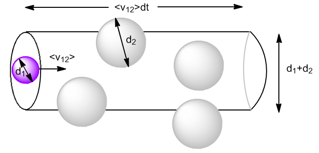
The kinetic theory allows us to calculate the frequency of collisions between molecules. We assume that the molecules are rigid spheres of diameter d and we neglect intermolecular forces except at the moment of collision. At high pressures, intermolecular forces cannot be neglected and the equations obtained are not applicable. We will use the following notation:
- $z_{12}$: number of collisions per unit time (frequency of collisions) that a molecule of gas 1 experiences with the molecules of gas 2.
- $z_{11}$: frequency of collisions that a molecule of gas 1 experiences with other molecules of gas 1.
- $Z_{12}$: total frequency of collisions between molecules of gas 1 with those of gas 2 per unit volume.
Let $N_1$ be molecules of gas 1 with diameter $d_1$ and $N_2$ be molecules of gas 2 with diameter $d_2$. Molecules move at average speeds $\bar{v}_1$ and $\bar{v}_2$.
We begin by calculating the collisions of type 1 with type 2 molecules $(z_{12})$. Let us consider the type 2 molecules at rest and the type 1 ones moving at velocity $\bar{v}_{12}$, the relative average speed of the type 1 molecules with respect to the type 2 ones.
- Details
- Written by: Germán Fernández
- Category: Kinetic theory of gases
- Hits: 1644
It is defined as the distance that a molecule advances between two successive collisions. Let $\bar{v}_1$ be the average speed of type 1 molecules. In a time t it travels a distance $\bar{v}_1t$ where the number of collisions is $[z_{11}+z_{12}] t$. Therefore, the average distance traveled by a molecule 1 between two collisions is: \begin{equation} \lambda=\frac{\bar{v}_1}{z_{11}+z_{12}} \end{equation} If the gas is pure: \begin{equation} \lambda=\frac{\bar{v}_1}{z_{11}}=\frac{1}{\sqrt{2}\pi d_1^2}\frac {V}{N_1} \end{equation} Using the equation PV=NkT, V/N=kT/P. \begin{equation} \lambda=\frac{1}{\sqrt{2}\pi d_1^2}\frac{kT}{P} \end{equation}