")
")
")
")
In this section we are going to deduce the equation that allows us to know the fraction of molecules that have the magnitude of their velocity between two determined values.
We call $dN_v/N$ the fraction of molecules with speed between v and v+dv. where N represents the total number of gas molecules. \begin{equation} \frac{N_v}{N}=G(v)dv \end{equation} G(v) is the velocity distribution function or probability density. By multiplying this function by $dv$, the fraction of molecules with speed between v and v+dv is obtained.
If we are interested in calculating the fraction of molecules with a velocity between $v_1$ and $v_2$, we integrate the velocity distribution function in that interval. (It is equivalent to talk about the fraction of molecules that have their speed in a given interval and the probability that a molecule has its speed included in said interval)
\begin{equation} P[v_1,v_2]=\int_{v_1}^{v_2 }G(v)dv \end{equation}
The probability that a molecule has its speed in the interval $[0,\infty]$ is 1
\begin{equation} \int_{0}^{\infty}G (v)dv=1 \end{equation}
To obtain G(v) we must integrate the function $\phi(\vec{v})=g(v_x)g(v_y)g(v_z)$ for a value v of the modulus of velocity through space. Since this integral extends over a spherical cap, it is convenient to use spherical coordinates ($v,\theta, \varphi$).
\begin{equation} g(v_x)g(v_y)g(v_z)dv_xdv_ydv_z=\left(\frac{m}{2\pi kT}\right)^{3/2}e^{-mv^2/ 2kT}dv_xdv_ydv_z \end{equation}
Making the change to spherical, $dv_xdv_ydv_z=v^2sin\theta dvd\theta d\varphi$, and integrating:
\begin{equation} \frac{dN_v}{N}=G(v )dv=\int_{0}^{\pi}\int_{0}^{2\pi}\left(\frac{m}{2\pi kT}\right)^{3/2}e^{ -mv^2/2kT}v^2sin\theta dvd\theta d\varphi \end{equation}
Since v and their differential are constants we can take them out of the integral.
\begin{equation} \frac{dN_v}{N}=G(v)dv=\left(\frac{m}{2\pi kT}\right)^{3/2}e^{-mv^2 /2kT}v^2dv\int_{0}^{\pi}\int_{0}^{2\pi}sin\theta d\theta d\varphi \end{equation}
\begin{equation} \frac{dN_v }{N}=G(v)dv=\left(\frac{m}{2\pi kT}\right)^{3/2}e^{-mv^2/2kT}v^2dv4\pi \end{equation}
Where the distribution function of the velocity magnitude G(v) is:
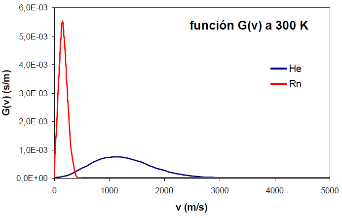
\begin{equation} G(v)=\left(\frac{m}{2\pi kT}\right)^{3 /2}e^{-mv^2/2kT}4\pi v^2 \end{equation}
At small values of the velocity module, the parabolic term ($v^2$) predominates and the function grows quadratically. At high values of v, the negative exponential $e^{-v^2}$ begins to dominate, causing the function G(v) to decrease its value, vanishing at infinity.
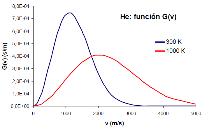
The increase in temperature produces a broadening in the distribution function and a displacement of its maximum at higher speeds.
An increase in the molecular mass, however, produces the opposite effect, narrowing of the function and displacement of its maximum at lower speeds.