")
")
")
")
Octave allows solving the equations of a kinetic system, in a very simple and efficient way. We will apply Octave to two complex kinetic systems: consecutive reactions and oscillating reactions (Lotka mechanism)
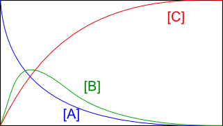
a) Consecutive reactions:
$A\stackrel{k_1}{\rightarrow} B \stackrel{k_2}{\rightarrow} C$, we solve the following differential equations with Octave: \begin{eqnarray} \frac{d[A]}{dt}& = & -k_1[A]\\ \frac{d[B]}{dt}& = & k_1[A]-k_2[B]\\ \frac{d[C]}{dt}& = & k_2[B ] \end{eqnarray}
We create a function that gives the velocity of the three components as a function of concentrations:
octave> function xdot = f(x,t) # x represents the concentrations of A, B and C, t is the time at a given instant and xdot are the derivatives of [A], [B] and [C] with respect to the time.
> global k # k is a vector representing the kinetic constants $k_1$ and $k_2$ is defined globally to be visible in the function above.
> xdot(1) = -k(1)*x(1) ; # define the first equation
> xdot(2) = k(1)*x(1) - k(2)*x(2); # define the second equation
> xdot(3) = k(2)*x(2); # define the third equation.
> end function
Now we go on to indicate the values of rate constants and initial concentrations:
octave> global k; k(1) = 1.0; k(2) = 1.0; # define k(1) and k(2)
octave> conc0(1) = 5.0; # define the initial concentration of A
octave> conc0(2) = 0.0; # define the initial concentration of B
octave> conc0(3) = 0.0; # defines the initial concentration of C
Next, we indicate the times between which we are going to carry out the integration and the number of stages that octave must carry out during the integration.
octave> t_initial = 0.0;
octave> t_final = 10.0;
octave> n_steps = 200;
octave> t = linspace(t_start, t_end, n_steps); # Integration of the differential equations is done by calling the lsode routine included in octave.
octave> conc = lsode("f", conc0, t); # The output is the matrix conc, whose columns are concentrations of the three components and time. However, a plot of concentrations versus times is more visual. We write the code that makes the graph:
octave> gset xlabel "time";
octave> gset ylabel "concentrations";
octave> plot(t, conc);
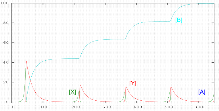
Lotka mechanism
$A+X\stackrel{k_1}{\rightarrow} 2X; \;\;\;\; X+Y\stackrel{k_2}{\rightarrow} 2Y; \;\;\;\; Y\stackrel{k_3}{\rightarrow}B$
The equations that give us the variations in time of the different reactants are: \begin{eqnarray} \frac{d[A]}{dt} & = & 0.0\\ \frac{d[X]}{dt} & = & k_1[A][X]-k_2[X][Y]\\ \frac{d[Y]}{dt} & = & k_2[X][Y]-k_3[Y]\\ \frac{ d[B]}{dt} & = & k_3[Y] \end{eqnarray}
We solve these equations numerically using octave.
octave> function xdot = f(x,t) # x represents the concentrations of A, X , Y and B, t is the time at a given instant and xdot are the derivatives of [A], [X], [Y] and [B] with respect to time.
> global k
> xdot(1) = 0.0; # define the first function
> xdot(2) = k(1)*x(1) *x(2) - k(2)*x(2)*x(3); # define the second function.
> xdot(3) = k(2)*x(2)*x(3) - k(3)*x(3); # define the third equation.
> xdot(4) = k(3)*x(3); # define the fourth equation.
> end function
octave> global k; k(1) = 0.05; k(2) = 0.1; k(3) =0.05; #$ define k(1) and k(2)
octave> conc0(1) = 5.0; # define the initial concentration of A
octave> conc0(2) = 5.0e-4; # define the initial concentration of X
octave> conc0(3) = 1.0e-5; #define the initial concentration of Y
octave> conc0(3) = 0.0; # define the initial concentration of B
octave> t_initial = 0.0;
octave> t_final = 650.0;
octave> n_steps = 10000;
octave> t = linspace(t_start, t_end, n_steps);
octave> conc = lsode("f", conc0, t);
octave> plot(t, conc);