")
")
")
")
Starting from the chemical potential of a solute according to the convention II
\begin{equation} \mu_{i}=\mu_{II,i}^{0}+RTln\gamma_{II,i}x_i \end{equation}
Molality of component i is given by, $m_i=\frac{n_i}{n_AM_A}$ where $M_A$ is the molecular weight of the solvent. Since the solvent is very abundant we can approximate the moles of A by the totals and suppose that, $x_i=\frac{n_i}{n_A}$. Substituting this mole fraction into the chemical potential equation
\begin{equation} \mu_i=\mu_{II,i}^{0}+RTln\left(\gamma_{II,i}m_ix_AM_A\frac{m^{0} }{m^{0}}\right) \end{equation}
In this last equation we multiply and divide by $m^0$ in order to separate the Neperian into two dimensionless addends.
\begin{equation} \mu_i=\underbrace{\mu_{II,i}^{0}+RTln(M_Am^0)}_{\mu_{m,i}^{0}}+RTln(\underbrace{ x_A\gamma_{II,i}}_{\gamma_{m,i}}m_i/m^0) \end{equation}
Therefore,
\begin{equation} \mu_{i}=\mu_{m,i }^{0}+RTln\gamma_{m,i}\frac{m_i}{m^0} \end{equation}
Where $\gamma_{m,i}\rightarrow 1$ when $x_A\rightarrow 1$ , $\gamma_{m,i}$ is the activity coefficient on the molality scale.
The normal chemical potential on the molality scale $\mu_{m,i}^{0}$ is defined as a fictitious state in which the molality of the solute in the solution is $m_i=1\;mol/kg$ and the solution behaves like an ideal dilute $\gamma_{m,i}\rightarrow 1$
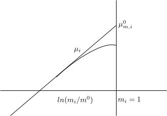
With $m_i$ small $\gamma_{m,i}\rightarrow 1$, ideal behavior and the graph is a straight line.
On the molar concentration scale, the chemical potential is written:
\begin{equation} \mu_i=\mu_{c,i}^{0}+RTln\left(\gamma_{c,i}\frac{c_i}{c ^0}\right) \end{equation}
Where, $c^{0}=1\;mol/dm^3$, also $a_{c,i}=\gamma_{c,i}\frac{c_ {i}}{c^0}$.