")
")
")
")
The probability of finding a molecule at a given energy level, j, is given by:
\begin{equation} p_j=\frac{e^{-\epsilon_j/kT}}{\sum e^{-\epsilon_i/kT}} \end{equation}
From the classical point of view, the kinetic energy of a molecule varies continuously and is given by the expression $\epsilon_x=\frac{1}{2}mv_x^2$. Taking this energy value to the probability expression, we obtain:
\begin{equation} dp(v_x)=\frac{dN_{v_x}}{N}=\frac{e^{-\frac{mv_x^2}{2kT}}dv_x}{\int_{-\infty} ^{\infty}e^{-\frac{mv_x^2}{2kT}}dv_x} \end{equation}
Where, $dp(v_x)$ represents the fraction of molecules with speed between $v_x$ and $v_x+dv_x$. The integral of the denominator represents the sum over all possible values of $v_x$ and has the form $\int e^{-bx}dx=(\pi/b)^{1/2}$
\begin{equation} dp(v_x)=\frac{dN_{v_x}}{N}=\frac{e^{-\frac{mv_x^2}{2kT}}dv_x}{\left(\frac{2 \pi kT}{m}\right)^{1/2}} \end{equation}
Given that $\frac{dN_{v_x}}{N}=g(v_x)dv_x$, the distribution function for $v_x$ is given by:
\begin{equation} g(v_x)=\left(\frac{m}{2\pi kT}\right)^{1/2}e^{-mv_{x}^{2}}/2kT \end{equation}
where m is the mass of a gas molecule, k is Boltzmann's constant, and T is the temperature.
The expressions for $g(v_y)$ and $g(v_z)$ are analogous given the equivalence between the spatial directions.
\begin{equation} g(v_x)=\left(\frac{m}{2\pi kT}\right)^{1/2}e^{-mv_{y}^{2}}/2kT \end{equation}
\begin{equation} g(v_x)=\left(\frac{m}{2\pi kT}\right)^{1/2}e^{-mv_{z}^{2}}/2kT \end{equation}
The units of the distribution function are inverse to those of the velocity, so that the probability obtained by multiplying it by $dv_x$ is dimensionless.
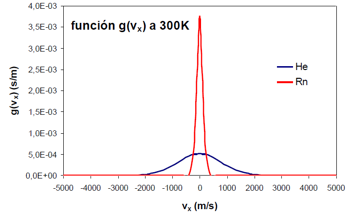
The function $g(v_x)$ is Gaussian, centered at $v_x=0$ and symmetric about the ordeand (y) axis. This symmetry means that the probability density of finding molecules at $v_x=a$ is equal to the probability of finding them at $v_x=-a$. The probability density reaches its maximum at zero, tending towards zero as $v_x$ goes towards $\pm \infty$.
An increase in the temperature of the gas produces an increase in the probability density for both positive and negative high values of the velocity.
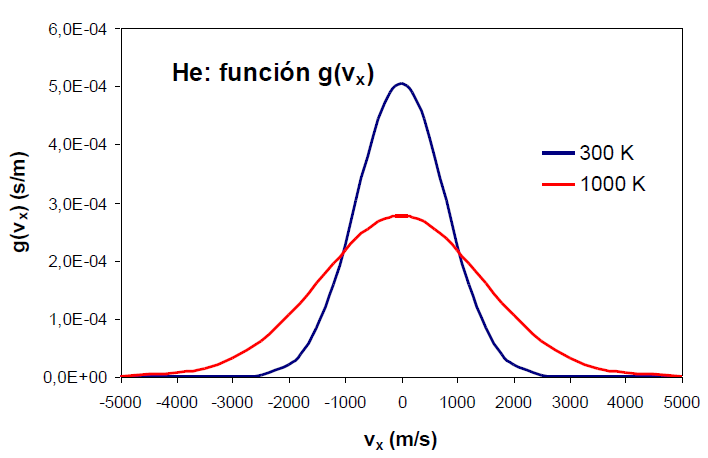
An effect similar to that of temperature can be observed by varying the mass of the gas. The following graph shows how as the mass of the gas decreases, the distribution function widens. Therefore, mass and temperature have opposite effects on the distribution function, a decrease in mass or an increase in temperature produce a broadening of the curve.